Calibrating
your Volksmeter
The Volksmeter
(VM) is an unusual
seismic instrument, having at its heart a
simple short pendulum. The general principle of operation is
straight forward, being a sensitive detector which measures the
displacement
of the pendulum, and which will therefore indicate either a tilt or
horizontal acceleration of the whole instrument. When
considering a modern automobile engine, the theory of
operation can get rather complex upon close inspection, and similarly
with 'simple' pendulums and how they behave. The inventor of the
Volksmeter is a particular authority on the motion of pendulums and has
written extensively on the subject. In an appendix to the
comprehensive Volksmeter
User
Manual, there is a detailed
theory
of
operation
covering seismometer detectors in general,
and pendulums in particular.
One of the useful features of acceleration sensors is
the ability to calibrate them by tilting them with respect to the
Earth's gravitational field, and so it is with the Volksmeter.
Because of its extreme sensitivity, particularly when operated in
24-bit mode, the Volksmeter can take quite some taming, and some
practice with setup is required. The technique for leveling the
VM is
covered quite
well in the on-line user manual in Chapter
2b.
Assuming that the reader has completed their Volksmeter's installation
at a
permanent site, and is operating it via WinSDR, there remains the
question of
what sensitivity figures should be entered into WinSDR's 'Sensor
information'
page, for both the acceleration channels (Channels 1 & 2) and
the velocity channels (Channels, 3 & 4). For Channels 1 &
2
this sensitivity figure represents the amount of horizontal
acceleration required to register a change of 1-bit by the VM's
detector.
WinSDR may be configured with various sensitivities by setting
the digitisation range anywhere between
16-bit to 24-bit operation. When operated in 24-bit mode the VM
is
very
sensitive
indeed and can be tricky to work with, due to flexure
of just about everything within and external to the instrument.
At these levels of sensitivity,
'hard' substances such as reinforced concrete floor support, can
effectively become a big slab of marshmallow.
The calibration process is relatively
straight forward, and utilises the VM's leveling screws. These
screws
are arranged in a triangle, with a single screw located on the left
hand side
(LHS) of the
instrument, and two screws on the right hand side (RHS). Consider
turning just the LHS leveling screw, which will cause
the whole instrument to tilt
about an axis running between the tips of the two RHS leveling
screws. Since we know that the thread pitch of the leveling
screws is 32 turns-per-inch, and the horizontal distance between the
LHS leveling screw tip and axis of rotation is 9.70 inches (246mm),
then a
single turn of the LHS screw will cause the whole instrument to tilt by
arctan(1/32"÷9.7")
=
0.185º
=
0.00322
radians.
When operated in 24-bit mode, the VM's digitiser output ranges between
±8,388,608 'counts'. In practice, and considering
just
Channel 2, it takes a little less than two complete turns of the LHS
screw to cause the digitiser output to range between the maximum -ve
counts and
maximum +ve counts. I have found that 1½ turns of the
LHS screw
can be comfortably accommodated within the 24-bit digitisation
span. Firstly
it is helpful to calculate the VM's counts/tilt ratio, normally
expressed in units of counts/radian. By adjusting the LHS screw
to a point
near maximum -ve counts, and then rotating it 1½ turns toward
+ve
counts, one can compute this ratio. For example, I adjusted the
LHS screw to a point where I read a figure of -7,129,000 counts, and
after rotating the screw 1½
turns anticlockwise, this figure became +7,670,000
counts. Taking the difference between these two and dividing by
1½,
yields
a
figure
of
around
9,866,000
counts/turn.
But one screw
turn changes the tilt by 0.00322
radians,
so
the
counts/radian
figure
for
my
particular
VM
is ≅2.0×10⁹
counts/radian. Note that this figure is for 24-bit digitisation,
and it will be reduced for
lower-resolution digitisation. For example, for 20-bit
digitisation it would be reduced by a factor of 16.
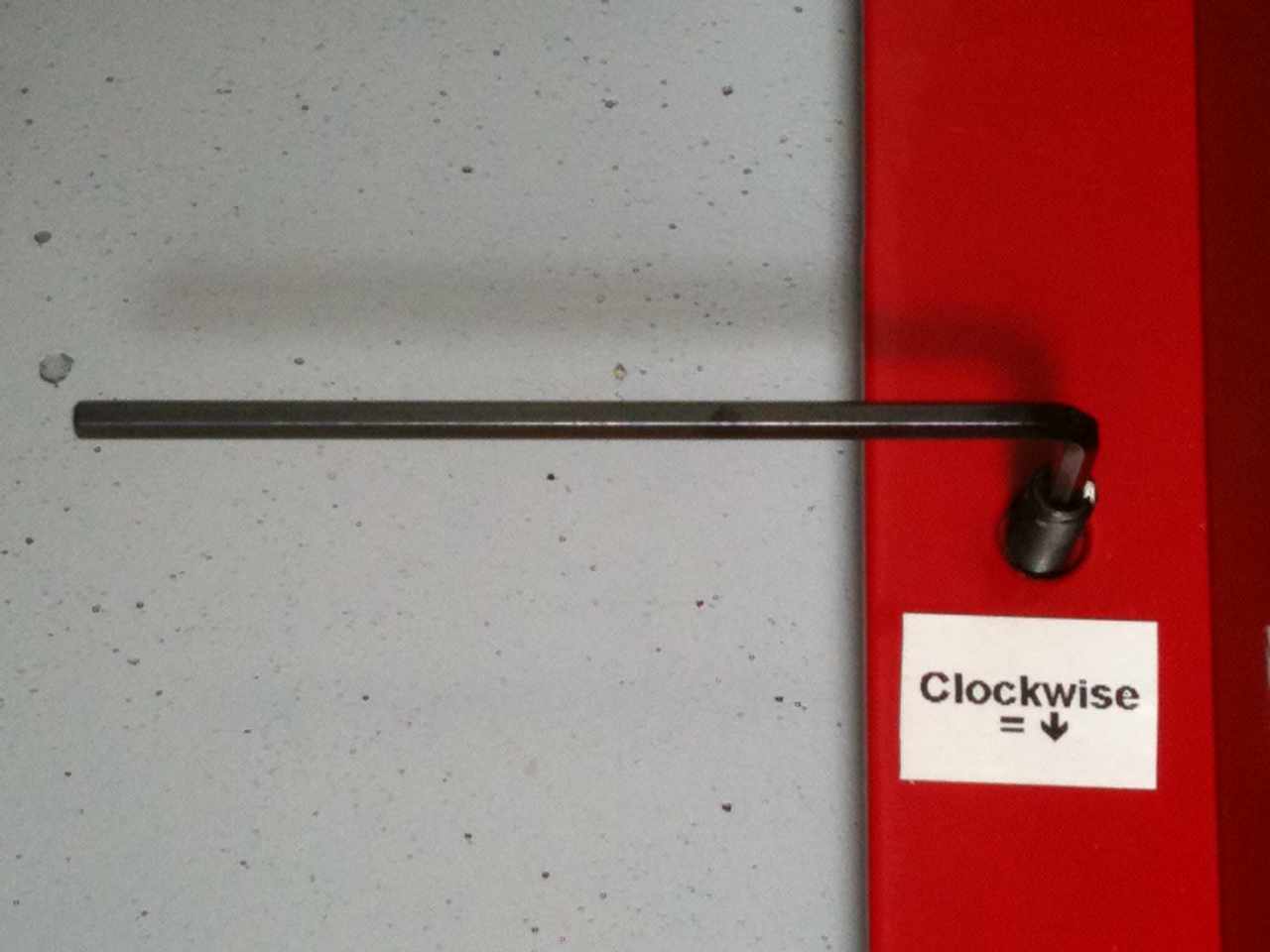 As a point of technique for accurately rotating a
leveling screw by 1½
turns
(or
any
other
amount),
I
recommend
placing
a tiny dot of white
paint (e.g. typewriter correction fluid) on the top of the screw to
indicate its general rotation position (it's easy to lose track of
rotation
otherwise). One may then use a 3/32"
Allan key to rotate the screw. As may be seen in the right-hand
image,
the
Allan
key
shaft
also
acts as an
analog pointer,
and
one
can
fairly
accurately
eyeball when the Allan key is pointing
directly away from the instrument or when it is aligned parallel with
the edge of the VM base plate. Another handy tip, which may also
be seen in this image, is to label the effect that screw rotation has
on WinSDR's screen trace. In this case, a clockwise rotation will
cause the WinSDR screen trace to move downwards (i.e. towards -ve
digitiser counts). This knowledge
can save a lot of mucking around when leveling the instrument.
As a point of technique for accurately rotating a
leveling screw by 1½
turns
(or
any
other
amount),
I
recommend
placing
a tiny dot of white
paint (e.g. typewriter correction fluid) on the top of the screw to
indicate its general rotation position (it's easy to lose track of
rotation
otherwise). One may then use a 3/32"
Allan key to rotate the screw. As may be seen in the right-hand
image,
the
Allan
key
shaft
also
acts as an
analog pointer,
and
one
can
fairly
accurately
eyeball when the Allan key is pointing
directly away from the instrument or when it is aligned parallel with
the edge of the VM base plate. Another handy tip, which may also
be seen in this image, is to label the effect that screw rotation has
on WinSDR's screen trace. In this case, a clockwise rotation will
cause the WinSDR screen trace to move downwards (i.e. towards -ve
digitiser counts). This knowledge
can save a lot of mucking around when leveling the instrument.
The standard textbook constant for 'g', the vertical acceleration due
to
Earth's gravity, is 9.80665m/s/s
(SI
units)
=
980.665cm/s/s
(cgs
units, used by WinSDR). A single rotation of the
LHS leveling screw will introduce a horizontal component of
acceleration of 1/32"÷9.7"x980.665
= 3.159cm/s/s. So in terms of acceleration/counts, for one turn
of the screw and 24-bit digitisation, the figure for my particular VM
is 3.159/9,866,000
≅
3.2x10⁻⁷cm/s/s/count,
which
is
the
required figure to enter
into WinSDR's
sensor
sensitivity
field (specifically enter "3.2e-007" into this
field). On the same setup page the 'Output Type' field needs to
be set
to 'Acceleration'. The
'Output
Voltage',
'Amp
Gain'
and
'A/D
Input' fields
don't apply to the VM and may be set to 0.0. Working on the
assumption that VM channels 1 & 2 have
similar performance,
I have set both my Channel 1 & 2 sensitivity fields to "3.2e-007".
This is well and good for the VM acceleration channels 1 & 2, but
what about the
VM velocity channels 3 and 4? What figure should be entered for
the sensor sensitivity here? This was a small puzzle for me for
quite some time, and I firstly tried the hit-and-miss adjustment
technique, by observing actual teleseismic quakes and by comparing my
measured peak ground velocities with those modeled by the USGS arrival
time calculator. This produced pleasingly consistent results,
but
still not exactly a calibrated value.
This puzzle was solved one day by the realisation that WinQuake has a
digital integration function, and it should therefore be possible
to digitally integrate one of the VM's acceleration channels, and to
compare it with a VM
channel which produces velocity output directly (e.g. integrated data
from VM Channel 1 should be very similar to that from Channel 3).
Exactly how WinSDR produces its real-time velocity channels (3 &
4), by performing a real-time integration of acceleration, is an
algorithmic 'black
box', but it seems to work well enough. If one takes a hour's
worth of VM acceleration data (say Channel 1, preferably containing
something interesting such as a teleseismic quake), and then
integrates it
via WinQuake, and then prints out the resultant trace, this visually
compares quite well with the trace of Channel 3 data acquired over the
same period. On close
inspection the two traces won't be exactly
the same, but usually pretty close, as may be seen with this
example showing integrated acceleration (upper trace) and
velocity (lower trace).
One thing to note when integrating data from VM Channels 1 & 2, is
that small consistent accelerations (i.e. tiny slow near-DC changes in
tilt occurring within the data period) can lead to some very peculiar
looking (e.g. banana
shaped) velocity traces. After
integrating VM
acceleration data, it is advisable to then apply a high-pass filter of
say 0.01Hz, to remove the near-DC components left over from integration.
WinQuake's 'Calculate
RMS' function may then be used to calculate the velocity
sensitivity figure. Firstly, enter a 'first guess' sensitivity
figure
for WinSDR channels 3 & 4 by entering "3.00e-007" into the
sensitivity fields. Then take a hour's worth of VM Channel 1
data, integrate it, filter it, and calculate the RMS velocity.
Then take the channel 3 data for the same period and calculate its RMS
velocity. These two RMS numbers will not match, but will likely
be
similar. For example, if the integrated acceleration [Channel 1]
RMS figure was 40um/s and the velocity [Channel 3] RMS was
30um/s, then Channel 3 velocity needs to be scaled up by a factor of
40/30. This would require multiplying the 'first guess'
sensitivity by 4/3, that is 3.0x10-7
x 4/3 = 4.00e-007 in
this case. With my particular VM instrument,
I have determined my Channel 3 & 4 sensitivity figure to be
"3.89e-007".
Each individual Volksmeter will need its own calibration,
but as an intermediate step to get a new VM owner up-and-running, I
suggest entering the following sensitivity constants into WinSDR's
sensor sensitivity fields.:
VM Channel
no.
|
Sensor
sensitivity
|
1
|
3.20e-007 |
2
|
3.20e-007 |
3
|
3.89e-007 |
4
|
3.89e-007 |
I would be interested to know what calibration figures other VM owners
have found, so please feel welcome to email me and I will post
the
results on this page.
2010-02-14